Fast Fourier Transformation
Given an $n$-dimensional vector $v \in \mathbb{C}^n$, its Discrete Fourier Transform $\mathcal{F}(v)$ is defined as the product of an $n \times n$ matrix $M_n$ (which will be introduced later) and the vector $v$:
The result is obtained by computing the vector product of each row of $M_n$ with $v$. Each row’s vector product takes $O(n)$ time, and since there are $n$ rows, the overall time complexity of the matrix multiplication is $O(n^2)$.
The Fast Fourier Transform algorithm reduces this to a time complexity of $O(n \log n)$ by using a divide-and-conquer approach.
Discrete Fourier Transform
Now we introduce the matrix $M_n$.
Consider the $n$-th roots of unity in the complex field $w$, i.e., $w^n = 1$, we have
Let $w_n$ be the $n$-th root of unity:
Let $w_n^{j,k}$ be the $j \times k$ power of $w_n$, where $j$ and $k$ denote the row and column indices, respectively. Note that the indices start from 0, i.e., $j, k = 0, 1, \ldots, n-1$.
The definition of the matrix $M_n$ is as follows:
To simplify the description, we assume that $n$ is a power of 2.
Fast Fourier Transform
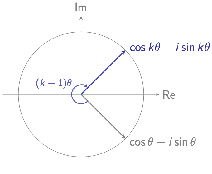
From Euler’s formula, we know that
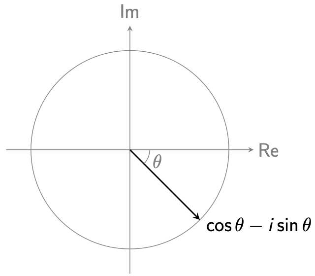
Let $\theta = \frac{2\pi}{n} $, then $w_n^k$ corresponds to rotating $w_n$ clockwise by $(k-1) \cdot \theta$ (as shown below):
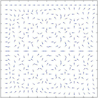
Now we can visualize $M_n$ in the following way. Taking $M_{16}$ as an example, it is illustrated below:
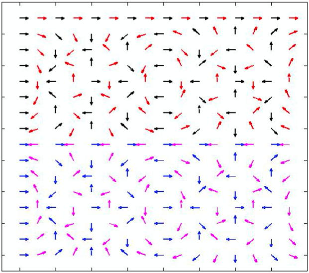
It seems a bit chaotic at the first glance. However, we can divide it into four submatrices, distinguished by four different colors, as shown below:
We observe that:
-
The black matrix and the blue matrix are identical, which is $M_8$;
-
Each red vector corresponds to rotating the black vector “to its left” clockwise, where the angle of rotation depends on the row of the vector.
Let the black element be $w_n^{ik}$, then the red element to its right is $w_n^{ik} \cdot w_n^i$. Thus, the red matrix can be expressed as
$$ M_8 \times u, \quad u= \begin{pmatrix} w_n^0\\ w_n^1\\ \vdots\\ w_n^{n-1} \end{pmatrix} = \begin{pmatrix} w^0_8\\ w^1_8\\ \vdots\\ w^7_8 \end{pmatrix}, $$ where $ \times $ denotes element-wise multiplication of each column in $M_8$ with $u$: $$ M_8\times u = \begin{bmatrix} w_8^{0,0}\cdot w_n^0 & w_8^{0,1}\cdot w_n^0 & \ldots & w_8^{0,7}\cdot w_n^0\\ w_8^{1,0}\cdot w_n^1 & w_8^{1,1} \cdot w_n^1 & \ldots & w_8^{1,7}\cdot w_n^1\\ & & \vdots &\\ w_8^{7,0} \cdot w_n^7& w_8^{7,1} \cdot w_n^7& \ldots & w_8^{7,7}\cdot w_n^7 \end{bmatrix} $$
-
The purple matrix has the opposite sign to the red matrix, i.e., $-M_8\times u$, which is equivalent to rotating the red vector 180 degrees clockwise.
Based on the above observations, we are about to derive the computation method for the Fast Fourier Transform.
First, we rearrange the columns of $M_n$, grouping even columns together and odd columns together. The new matrix is denoted by $\bar{M}_n$:
Correspondingly, we also need to rearrange the elements in $v$ by index, separating even and odd positions.
The new vector is denoted by $ \bar{v}_n $:
Thus, we have
That is,
This is the Fast Fourier Transform algorithm, which can be implemented as below.
def FFT(v):
    “”“ Fast Fourier Transform.
    ”“”
    n = len(v)
    if n == 1:
        return v
    v_even = FFT(v[0:n:2])
    v_odd = FFT(v[1:n:2])
    u = [w_n**i for i in range(n//2)]
    part1 = [v_even[i] + u[i]*v_odd[i] for i in range(n//2)]
    part2 = [v_even[i] - u[i]*v_odd[i] for i in range(n//2)]
    return part1 + part2
Next, we analyze the computational complexity.
Let $T(n)$ represent the computation time for the discrete Fourier transform of a vector of length $n$. According to the above formula, calculating $\mathcal{F}(v_{\text{even}})$ and $\mathcal{F}(v_{\text{odd}})$ takes $T(n/2)$ time each, with the concatenation taking $O(n)$ time. We have:
The Inverse Transform
Let’s take another look at the inverse of the fast Fourier transform.
We observe that
This yields
Here, $\sigma_{n-1}(v)$ represents the last $n-1$ elements of vector $v$ arranged in reverse order by index.
Noticing that $\sigma_{n-1}(\sigma_{n-1}(v)) = v$, we have
That is,
Here is the Python implementation.
def iFFT(v):
    """ Inverse of the Fast Fourier Transform.
    """
    n = len(v)
    u = FFT(v)
    x = [i/n for i in u]  # u divided by n
    # Reverse the last n-1 elements
    y = x[1:]
    y.reverse()
    return x[0:1] + y